
Tim Abraham
The Gambler’s Ruin: A Simple Explanation and Derivation
I’ve recently had the itch to break out some textbooks and do a little math. Don’t ask me where that desire comes from, but I find working on math problems fun. A few years ago I bought a probability textbook, which I learned about through an Amazon review by my intellectual hero, Nassim Taleb (here’s the review). Since then it has mainly been sitting on my book shelf, but occasionally I leaf through it and try to refresh my memory on some concept or learn a new one.
In the book, I came across a very famous problem in probability called The Gambler’s Ruin. In the problem, we have the following scenario:
Two players, Player A and Player B, play a series of consecutive gambling games until one of the players loses all their money. Player A starts with a dollars and Player B starts with b dollars and the loser pays one dollar to the winner in each game. Player A’s chance of winning a game is \(p\) and Player B’s chance is \(q\) (where \(p+q=1\)). What is the probability, at any level of wealth Player A is at, that he will be ruined?
It’s not hard to find a solution for this problem online. I even found an okay explanation of it by the author of my textbook on YouTube. However, I was a bit rusty on some of my math and found all the answers out there to be a bit hand wavy in their derivations. They go through the most confusing steps with no explanation, which was frustrating for me. I like simple, straightforward explanations. And since I couldn’t find a single one on the Internet, I decided to contribute it myself. So let’s walk through the problem, very slowly, step by step. If you follow me with a pencil and paper I guarantee you’ll be able to understand the math. My goal is to be as comprehensive and thorough as possible.
The Setup
How do you even start with this problem? The question above asks “What is the probability, at any level of wealth Player A is at, that he will be ruined?”. So let’s call this \(P_n\). \(P_n\) is the probability that when Player A has n dollars, he will ultimately be ruined. How does Player A get to a position where he has n dollars? Well there are two ways he can get there: He can either lose a game when he has n + 1, or he can win a game when he has n - 1. We know the probability of him winning and losing a game is \(p\) and \(q\), respectively, and we know these are mutually exclusive events. Therefore, we can write out the equation for \(P_n\) as
- \[P_n=pP_{n+1}+qP_{n-1}\]
We get there by applying the theorem of total probability if you want to start at first principles, but I think the equation makes sense without any more set up. So we have our equation to solve!
Initial conditions
Two initial conditions can help us solve the problem. \[P_0=1\] This says that when Player A has $0, he is ruined. When Player A runs out of money, he can no longer play the game, so he’s stuck in this state. His probability of ruin is therefore 1, since he has no chance of getting back in the action. \[P_{a+b}=0\] This says the opposite. If Player A has won both his $a and Player B’s $b, he has won all the dollars. Player B can no longer play, so the game is over and Player A has no chance of being ruined.
Solving a difference equation.
Equation (1) is known as a difference equation. I haven’t solved too many of them, or at least been aware that I was, and maybe you’re in the same boat. We can rewrite equation (1) as
- \[p(P_{n+1}-P_n) = q(P_n-P_{n-1})\]
or \[P_{n+1}-P_n=\frac{q}{p}(P_n-P_{n-1})\].
Hopefully you’re still with me. All we did to get (2) was use the fact that \(p+q=1\) and multiply the left hand side \(P_n\) by \((p+q)\). The next part of the solution I got stuck on a bit. In most of the derivations I saw, we go from the above equation, to
- \[P_{n+1}-P_n=\frac{q}{p}(P_n-P_{n-1})=(\frac{q}{p})^n(P_1-1)\]
Huh? How’d we get there? Let me show you. Let’s try plugging in some numbers. First let’s say \(n=1\). Plug that into (3)
\[P_2-P_1=\frac{q}{p}(P_1-P_0)\] But we know from our initial conditions that \(P_0=1\), so: \[P_2-P_1=\frac{q}{p}(P_1-1)\]
Great, now let’s try for \(n=2\). Plugged into (3) gives \[P_3-P_2=\frac{q}{p}(P_2-P1)\]
You can see a pattern emerging here. But you can also see that the \((P_2-P_1)\) in the above equation was already solved for in the \(n=1\) scenario. So we can simply plug that in. \[P_3-P_2=\frac{q}{p}\frac{q}{p}(P_1-1)=(\frac{q}{p})^2(P_1-1)\]
Now consider the general case with \(n\). Feel free to try with \(n=3\) if you haven’t gotten the pattern. If you keep iterating, you’ll continue to wind up with something that equals \((\frac{q}{p})^n(P_1-1)\).
Fun with Geometric Sequences
Let’s take another route now. We’ve simplified \(P_{n+1}-P_n\), but what about when we’re not just looking at a difference of 1 game? Let’s exploit our other initial condition of \(P_{a+b}=1\) and solve for \(P_{a+b}-P_n\). Again, let’s plug in some numbers. Let’s say \(n=1\) and \(a+b=3\). Now we have \(P_3-P_1\). From the work we did above we know \(P_3-P_2\) and \(P_2-P_1\), and adding those together gives us \(P_3-P_1\). We could also write that as
\[P_3-P_1=\sum\limits_{k=1}^{2}P_{k+1}-P_k\]
Or more generally \[P_{a+b}-P_{n}=\sum\limits_{k=n}^{a+b-1}P_{k+1}-P_k\].
We can plug in our solution for \(P_{n+1}-P_n\) from (3) into the \(P_{k+1}-P_k\) and get
- \[=\sum\limits_{k=n}^{a+b-1}(\frac{q}{p})^k(P_1-1) \]
Now we’d like to get rid of that summation term. This is a geometric series, so there’s a very cool trick we can perform here to get find what that summation is equal to. I had completely forgotten about learning this trick in grad school. Like I said, my math is very rusty and I’m sure yours is too. So here’s how you solve for it. Let’s call the sequence \(\sum\limits_{k=n}^{a+b-1}(\frac{q}{p})^k=S_k\). Okay, let’s start expanding it out:
- \[S_k=\frac{q}{p}^n+\frac{q}{p}^{n+1}+...+\frac{q}{p}^{a+b-1}\]
Now the trick, where we multiply each side by \(\frac{q}{p}\).
- \[\frac{q}{p}S_k=\frac{q}{p}^{n+1}+\frac{q}{p}^{n+2}+...+\frac{q}{p}^{a+b}\]
And let’s subtract (6) from (5). Almost all the terms on the right hand side cancel out.
\[ S_k - \frac{q}{p}S_k =\frac{q}{p}^n - \frac{q}{p}^{a+b} \]
\[ (1-\frac{q}{p})S_k =\frac{q}{p}^n - \frac{q}{p}^{a+b} \]
\[ S_k =\frac{\frac{q}{p}^n - \frac{q}{p}^{a+b}}{1-\frac{q}{p}} \]
Very cool, right? We can plug that back in for the summation in (4) and get
- \[P_{a+b}-P_{n}=(P_1-1)\frac{\frac{q}{p}^n - \frac{q}{p}^{a+b}}{1-\frac{q}{p}}\]
Home stretch!
We’re basically home free now. Recall that \(P_{a+b}=0\) and then multiply both sides by \(-1\) to get
- \[P_n=(1-P_1)\frac{\frac{q}{p}^n - \frac{q}{p}^{a+b}}{1-\frac{q}{p}}\]
We’ve almost written this in terms of only n,a, and b, but we still don’t know what \((1-P_1)\) is. We can take care of that by using the other initial condition again \(P_0=1\).
\[\begin{equation} P_0=(1-P_1)\frac{\frac{q}{p}^0 - \frac{q}{p}^{a+b}}{1-\frac{q}{p}}=1 \end{equation}\]
We can now divide (8) by 1.
\[P_n=\frac{(1-P_1)}{(1-P_1)}\frac{(\frac{q}{p}^n - \frac{q}{p}^{a+b})(1-\frac{q}{p})}{(\frac{q}{p}^0 - \frac{q}{p}^{a+b})(1-\frac{q}{p})}\]
Which you can see a lot can be cancelled out from. Also, \(\frac{q}{p}^0=1\). That gives us \[P_n=\frac{(\frac{q}{p})^n - (\frac{q}{p})^{a+b}}{1-(\frac{q}{p})^{a+b}}\]
And if we substitute \(n=a\), we can then factor out a \(\frac{q}{p}^{a+b}\) from the numerator and denominator and we’ll get the probability of ruin for player A when his wealth is a.
\[P_a=\frac{1 - \frac{p}{q}^b}{1-\frac{p}{q}^{a+b}}\]
Which is our answer! That’s quite a bit of math, but laid out step by step with explanations it’s very straightforward. Now that we’ve got our solution, let’s build some intuition around that last equation and simulate some gambling scenarios.
Intuition and moral of The Gambler’s Ruin
The earliest mention of this problem was in a letter from Blaise Pascal to Pierre Fermat in 1656. That was obviously pre-Vegas. Today, the problem is often used as a cautionary tale for anyone naive enough to think they can beat the house on their next trip to the casino. As we’ll see with some simulations, as long as the odds are slightly not in your favor, you will always go broke. And when you’re playing against a rich opponent, like say, a deep pocketed casino, you’re basically fucked.
So moral of the story: If you’re playing a gambling game like the one described in this problem, quit while (and if) you’re ahead. Roulette is probably the most relevant game to this problem. Roulette has nearly symmetric payout odds, with the odds just slightly tipped towards the house. If you go to Vegas and play one dollar roulette, you will eventually go broke. The same is true for any game in the casino, except for poker.
Let’s Simulate!
I find the best way to build intuition on a tough mathematical result is to run some simulations. We’ve got our solution for \(P_a\) in terms of the win probabilities p and q and the total capital the players are currently at, which are a and b.
So let’s play around with these values. The formula is pretty easy to write in a programming language - I’ll use R here.
prob_ruin_a <- function(a, b, p) {
  # probability of Player B winning is q
  q = 1 - p # since p + q have to = 1

  # The ratio of q/p, which we used in the solution
  ratio = p/q

  # Numerator of the solution
  num = 1 - ratio^b

  # and Denominator
  den = 1 - ratio ^ (a + b)

  return(num / den)
}
Let’s try a few values. First let’s make the game only slightly in favor of player B but give him more and more wealth.
library(tidyverse)## ── Attaching packages ─────────────────────────────────────── tidyverse 1.3.2 ──
## ✔ ggplot2 3.4.2 ✔ purrr 1.0.1
## ✔ tibble 3.2.1 ✔ dplyr 1.1.2
## ✔ tidyr 1.3.0 ✔ stringr 1.5.0
## ✔ readr 2.1.4 ✔ forcats 0.5.2
## ── Conflicts ────────────────────────────────────────── tidyverse_conflicts() ──
## ✖ dplyr::filter() masks stats::filter()
## ✖ dplyr::lag() masks stats::lag()b_wealth <- c(50, 60, 100, 200, 500, 1000)
b_wealth %>% map_dbl(prob_ruin_a, a = 50, p = 0.499)## [1] 0.5498341 0.5994213 0.7306926 0.8711488 0.9724110 0.9966294We’re giving almost equal odds. Player A will win the game 49.9% of the time. When they both start with $50, the chances of ruin for Player A not too bad at 55%. But even with Player B having $100, the probability of ruin for A is already at 73%, and if B has $1000 the probability of ruin is 99.7%! At $1000, Player B simply has too much in reserve for Player A to stand a chance.
Using a bunch of values for Player B’s wealth from $50 to $1000, we can see the probability of ruin for Player A increases exponentially.
b_wealth <- seq(50, 1000, by = 10)
a_out_b_wealth <- b_wealth %>% map_dbl(prob_ruin_a, a = 50, p = 0.499)

data_frame(b_wealth, p = a_out_b_wealth) %>%
  ggplot(aes(b_wealth, p)) + geom_line(color = 'darkred') +
labs(y = 'Probability of Ruin for Player A', x = 'Wealth of Player B', title = 'Player A starts with $50') 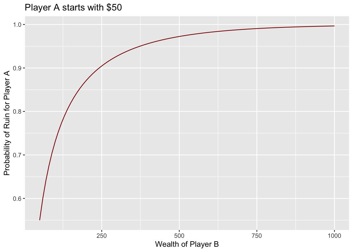
And that’s when the odds are almost even! Let’s now keep Player A and Player B’s wealth both at $50, but let’s change p, the probability Player A has of winning a game.
prob_p <- seq(.1, .49, by = 0.01)
prob_ruins <- prob_p %>% map_dbl(prob_ruin_a, a = 50, b = 50)
data_frame(prob_p, prob_ruins) %>%
  ggplot(aes(prob_p, prob_ruins)) + geom_line(color = 'darkred') +
labs(y = 'Probability of Ruin for Player A', x = 'Probability of Player A winning a game (p)', title = 'Both Players start with $50') 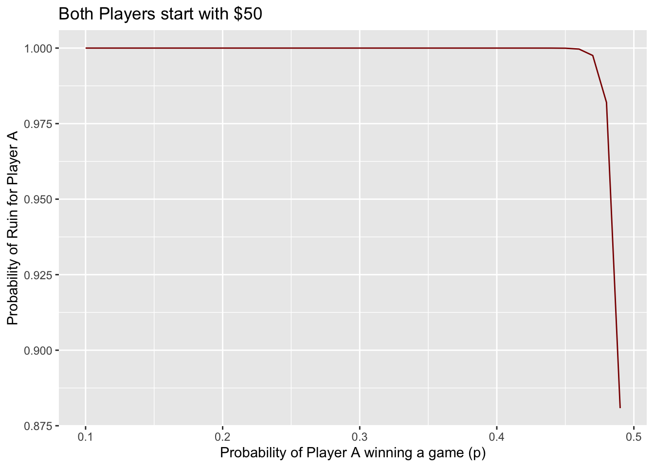
Yikes! Even if they have the same amount to begin with, even a slight unbalance in \(p/q\) spells disaster for Player A. A 48% chance of winning a game leads to a 98% chance of ruin!
Conclusion
In conclusion, even if you think you are “lucky” or somehow naively believe you are skilled at games of chance, stay away from anything that resembles this problem in the real world.
Hope you found the math easy to follow and let me know in the comments if you have any questions!